Extending mlr3 to time series forecasting.
This package is in an early stage of development and should be considered experimental. If you are interested in experimenting with it, we welcome your feedback!
Installation
Install the development version from GitHub:
# install.packages("pak")
pak::pak("mlr-org/mlr3forecast")
Usage
The goal of mlr3forecast is to extend mlr3 to time series forecasting. This is achieved by introducing new classes and methods for forecasting tasks, learners, and resamplers. For now the forecasting task and learner is restricted to time series regression tasks, but might be extended to classification tasks in the future.
We support both traditional forecasting learners (e.g., ARIMA, ETS) and machine learning forecasting, i.e. using regression learners with lag features for recursive one-step-ahead prediction.
Example: forecasting with forecast learner
Native forecasting learners are provided by packages such as forecast, smooth, prophet, and tscount.
library(mlr3forecast)
library(mlr3pipelines)

task = tsk("airpassengers")
task
#>
#> ── <TaskFcst> (144x1): Monthly Airline Passenger Numbers 1949-1960 ─────────────
#> • Target: passengers
#> • Properties: ordered
#> • Order by: month
#> • Frequency: month

# or plot the task
autoplot(task)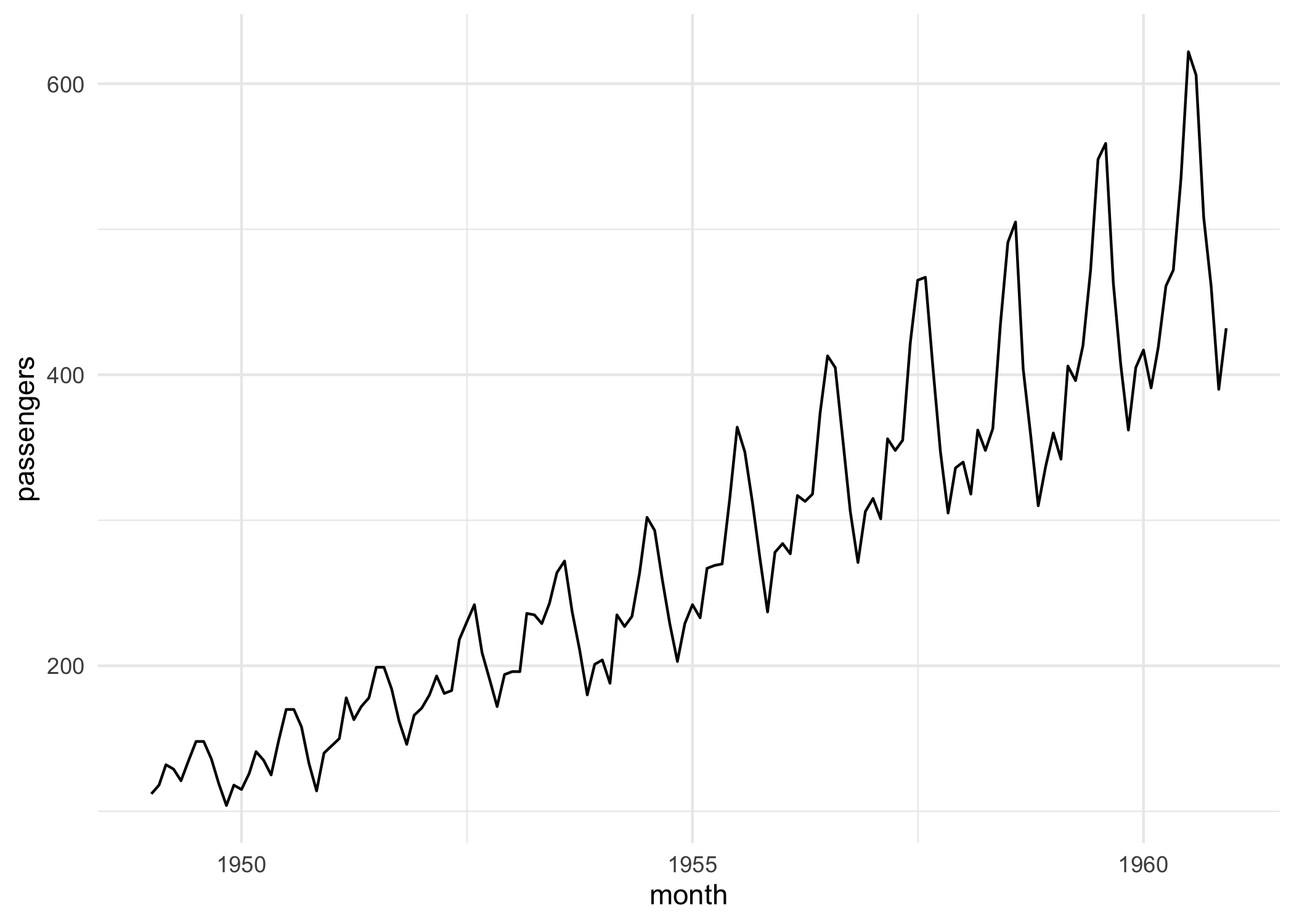
# train a forecast learner
learner = lrn("fcst.auto_arima")$train(task)
prediction = learner$predict(task, 140:144)
prediction
#>
#> ── <PredictionRegr> for 5 observations: ────────────────────────────────────────
#>  row_ids truth response      month
#>      140   606 623.9219 1960-08-01
#>      141   508 513.8585 1960-09-01
#>      142   461 450.7762 1960-10-01
#>      143   390 410.8961 1960-11-01
#>      144   432 439.9462 1960-12-01
prediction$score(msr("regr.rmse"))
#> regr.rmse
#>  13.85518

# generate new data to forecast unseen data
newdata = generate_newdata(task, 12L)
head(newdata)
#>         month passengers
#> 1: 1961-01-01         NA
#> 2: 1961-02-01         NA
#> 3: 1961-03-01         NA
#> 4: 1961-04-01         NA
#> 5: 1961-05-01         NA
#> 6: 1961-06-01         NA
prediction = learner$predict_newdata(newdata, task)
prediction
#>
#> ── <PredictionRegr> for 12 observations: ───────────────────────────────────────
#>  row_ids truth response      month
#>        1    NA 445.6351 1961-01-01
#>        2    NA 420.3953 1961-02-01
#>        3    NA 449.1988 1961-03-01
#>      ---   ---      ---        ---
#>       10    NA 494.1275 1961-10-01
#>       11    NA 423.3336 1961-11-01
#>       12    NA 465.5085 1961-12-01

# add a target log transformation
learner = as_learner(ppl(
  "targettrafo",
  graph = lrn("fcst.auto_arima"),
  targetmutate.trafo = function(x) log(x),
  targetmutate.inverter = function(x) list(response = exp(x$response))
))
prediction = learner$train(task)$predict(task, 140:144)
prediction$score(msr("regr.rmse"))
#> regr.rmse
#>  12.29896

# works with quantile response
learner = lrn(
  "fcst.auto_arima",
  predict_type = "quantiles",
  quantiles = c(0.1, 0.15, 0.5, 0.85, 0.9),
  quantile_response = 0.5
)$train(task)
learner$predict_newdata(newdata, task)
#>
#> ── <PredictionRegr> for 12 observations: ───────────────────────────────────────
#>  row_ids truth     q0.1    q0.15     q0.5    q0.85     q0.9 response      month
#>        1    NA 430.8905 433.7106 445.6351 457.5595 460.3796 445.6351 1961-01-01
#>        2    NA 403.0907 406.4005 420.3953 434.3901 437.6999 420.3953 1961-02-01
#>        3    NA 429.7726 433.4882 449.1988 464.9093 468.6249 449.1988 1961-03-01
#>      ---   ---      ---      ---      ---      ---      ---      ---        ---
#>       10    NA 469.8626 474.5036 494.1275 513.7514 518.3925 494.1275 1961-10-01
#>       11    NA 398.8383 403.5234 423.3336 443.1438 447.8290 423.3336 1961-11-01
#>       12    NA 440.8230 445.5445 465.5085 485.4725 490.1940 465.5085 1961-12-01

# resampling
learner = lrn("fcst.auto_arima")
resampling = rsmp("fcst.holdout", ratio = 0.7)
rr = resample(task, learner, resampling)
rr$aggregate(msr("regr.rmse"))
#> regr.rmse
#>   27.1211
Example: forecasting with regression learner
library(mlr3learners)

task = tsk("airpassengers")
learner = lrn("regr.ranger")
flrn = as_learner_fcst(learner, lags = 1:12)$train(task)
newdata = generate_newdata(task, 12L)
prediction = flrn$predict_newdata(newdata, task)
prediction
#>
#> ── <PredictionRegr> for 12 observations: ───────────────────────────────────────
#>  row_ids truth response      month
#>        1    NA 437.2866 1961-01-01
#>        2    NA 437.8537 1961-02-01
#>        3    NA 456.2050 1961-03-01
#>      ---   ---      ---        ---
#>       10    NA 478.8000 1961-10-01
#>       11    NA 440.9520 1961-11-01
#>       12    NA 442.7185 1961-12-01
prediction = flrn$predict(task, 140:144)
prediction
#>
#> ── <PredictionRegr> for 5 observations: ────────────────────────────────────────
#>  row_ids truth response      month
#>      140   606 574.6659 1960-08-01
#>      141   508 501.3702 1960-09-01
#>      142   461 453.8858 1960-10-01
#>      143   390 413.3260 1960-11-01
#>      144   432 428.7291 1960-12-01
prediction$score(msr("regr.rmse"))
#> regr.rmse
#>  18.06208

flrn = as_learner_fcst(learner, lags = 1:12)
resampling = rsmp("fcst.holdout", ratio = 0.9)
rr = resample(task, flrn, resampling)
rr$aggregate(msr("regr.rmse"))
#> regr.rmse
#>  49.58838

resampling = rsmp("fcst.cv")
rr = resample(task, flrn, resampling)
rr$aggregate(msr("regr.rmse"))
#> regr.rmse
#>  26.98398
By default as_learner_fcst() builds a recursive forecaster (one model, applied iteratively). Pass strategy = "direct" together with horizons to train one model per horizon — predictions then come straight from each horizon’s model, with no error accumulation:
task = tsk("airpassengers")
flrn = as_learner_fcst(
  lrn("regr.ranger"),
  lags = 1:12,
  strategy = "direct",
  horizons = 12
)$train(task, 1:132)
flrn$predict(task, 133:144)$score(msr("regr.rmse"))
#> regr.rmse
#>  71.18526
Or with some feature engineering using mlr3pipelines:
library(mlr3pipelines)

task = tsk("airpassengers")
task$set_col_roles("month", add = "feature")
graph = po("fcst.lags", lags = 1:12) %>>%
  po(
    "datefeatures",
    param_vals = list(
      week_of_year = FALSE,
      day_of_year = FALSE,
      day_of_month = FALSE,
      day_of_week = FALSE
    )
  ) %>>%
  lrn("regr.ranger")
flrn = as_learner_fcst(graph)$train(task)
prediction = flrn$predict(task, 142:144)
prediction$score(msr("regr.rmse"))
#> regr.rmse
#>  14.35202
Use selector_fcst_lags() to apply transformations only to the lag features, e.g. log-transforming lags while leaving date features untouched:
task = tsk("airpassengers")
task$set_col_roles("month", add = "feature")
graph = po("fcst.lags", lags = 1:12) %>>%
  po("colapply", applicator = log, affect_columns = selector_fcst_lags()) %>>%
  po(
    "datefeatures",
    param_vals = list(
      week_of_year = FALSE,
      day_of_year = FALSE,
      day_of_month = FALSE,
      day_of_week = FALSE
    )
  ) %>>%
  lrn("regr.ranger")
flrn = as_learner_fcst(graph)$train(task)
prediction = flrn$predict(task, 142:144)
prediction$score(msr("regr.rmse"))
#> regr.rmse
#>  13.21976
Target transformations can be applied by wrapping the forecast learner in ppl("targettrafo"). The lags are created from the transformed target and predictions are automatically inverted back to the original scale:
task = tsk("airpassengers")
graph = po("fcst.lags", lags = 1:12) %>>% lrn("regr.ranger")
pipeline = ppl(
  "targettrafo",
  graph = as_learner_fcst(graph),
  targetmutate.trafo = function(x) log(x),
  targetmutate.inverter = function(x) list(response = exp(x$response))
)
learner = as_learner(pipeline)$train(task)
prediction = learner$predict(task, 142:144)
prediction$score(msr("regr.rmse"))
#> regr.rmse
#>  14.40983
Example: comparing classical and ML forecasters
ML forecasters declare task_type = "fcst", so they can be benchmarked side-by-side with classical learners on the same task in a single benchmark() call:
task = tsk("airpassengers")
resampling = rsmp("fcst.holdout", ratio = 0.9)$instantiate(task)
n_test = length(resampling$test_set(1L))

learners = list(
  lrn("fcst.arima"),
  as_learner_fcst(lrn("regr.ranger"), lags = 1:12),
  as_learner_fcst(lrn("regr.ranger"), lags = 1:12, strategy = "direct", horizons = n_test)
)
design = benchmark_grid(task, learners, resampling)
bmr = benchmark(design)
bmr$aggregate(msr("regr.rmse"))[, .(learner_id, regr.rmse)]
#>               learner_id regr.rmse
#> 1:            fcst.arima 216.31005
#> 2: fcst.lags.regr.ranger  47.46578
#> 3:           regr.ranger  77.96068
Example: ensemble forecasting
Forecast learners produce regression predictions under the hood, so the standard mlr3pipelines ensemble pattern works directly: branch to several forecasters with gunion() and average their forecasts with po("regravg"). This mirrors the idea behind the forecastHybrid package, but with any mix of classical or ML learners.
task = tsk("airpassengers")

graph = gunion(list(
  po("learner", lrn("fcst.auto_arima"), id = "arima"),
  po("learner", lrn("fcst.ets"), id = "ets"),
  po("learner", lrn("fcst.theta"), id = "theta")
)) %>>%
  po("regravg")
flrn = as_learner(graph)$train(task)
forecast(flrn, task, 12L)
#>
#> ── <PredictionRegr> for 12 observations: ───────────────────────────────────────
#>  row_ids truth response
#>        1    NA 442.5050
#>        2    NA 427.6327
#>        3    NA 478.5120
#>      ---   ---      ---
#>       10    NA 471.2626
#>       11    NA 408.0117
#>       12    NA 455.0409
flrn$predict(task, 140:144)$score(msr("regr.rmse"))
#> regr.rmse
#>  12.23143

# weight the members instead of averaging equally
graph$param_set$set_values(regravg.weights = c(0.5, 0.3, 0.2))
flrn = as_learner(graph)$train(task)
flrn$predict(task, 140:144)$score(msr("regr.rmse"))
#> regr.rmse
#>  12.28049
Example: tuning a forecaster
Forecast learners are regular mlr3 learners, so they plug into the standard mlr3tuning machinery. Mark hyperparameters with to_tune() and wrap the learner in an auto_tuner(), using a forecasting resampling such as fcst.holdout or fcst.cv to respect the temporal order:
library(mlr3tuning)

task = tsk("airpassengers")

# tune an ML forecaster
flrn = as_learner_fcst(lrn("regr.ranger"), lags = 1:12)
flrn$param_set$set_values(
  regr.ranger.mtry.ratio = to_tune(0.1, 1),
  regr.ranger.num.trees = to_tune(100, 500)
)
at = auto_tuner(
  tuner = tnr("random_search"),
  learner = flrn,
  resampling = rsmp("fcst.cv"),
  measure = msr("regr.rmse"),
  term_evals = 4
)
at$train(task)
at$tuning_result[, .(regr.ranger.mtry.ratio, regr.ranger.num.trees, regr.rmse)]
#>    regr.ranger.mtry.ratio regr.ranger.num.trees regr.rmse
#> 1:              0.7511458                   427   16.1781

# the AutoTuner is itself a learner: predict with the best configuration
at$predict(task, 142:144)$score(msr("regr.rmse"))
#> regr.rmse
#>  7.522027
Classical forecasters tune the same way:
flrn = lrn("fcst.auto_arima")
flrn$param_set$set_values(stationary = to_tune(p_lgl()), seasonal = to_tune(p_lgl()))
at = auto_tuner(
  tuner = tnr("grid_search"),
  learner = flrn,
  resampling = rsmp("fcst.holdout", ratio = 0.8),
  measure = msr("regr.rmse")
)
at$train(task)
at$tuning_result[, .(stationary, seasonal, regr.rmse)]
#>    stationary seasonal regr.rmse
#> 1:      FALSE     TRUE  35.08279
Example: forecasting electricity demand
library(mlr3learners)
library(mlr3pipelines)

task = tsk("electricity")
task$set_col_roles("date", add = "feature")
graph = po("fcst.lags", lags = 1:3) %>>%
  po("datefeatures", param_vals = list(year = FALSE)) %>>%
  lrn("regr.ranger")
flrn = as_learner_fcst(graph)$train(task)

max_date = task$data()[.N, date]
newdata = data.table(
  date = max_date + 1:14,
  demand = rep(NA_real_, 14L),
  temperature = 26,
  holiday = c(TRUE, rep(FALSE, 13L))
)
prediction = flrn$predict_newdata(newdata, task)
prediction
#>
#> ── <PredictionRegr> for 14 observations: ───────────────────────────────────────
#>  row_ids truth response       date
#>        1    NA 187397.2 2015-01-01
#>        2    NA 195770.3 2015-01-02
#>        3    NA 188009.8 2015-01-03
#>      ---   ---      ---        ---
#>       12    NA 222302.3 2015-01-12
#>       13    NA 226607.9 2015-01-13
#>       14    NA 227931.6 2015-01-14
Example: global forecasting
library(mlr3learners)
library(mlr3pipelines)
library(tsibble)

dt = setDT(tsibbledata::aus_livestock)
setnames(dt, tolower)
dt[, month := as.Date(month)]
dt = dt[, .(count = sum(count)), by = .(state, month)]
setorder(dt, state, month)
task = as_task_fcst(dt, id = "aus_livestock", target = "count", order = "month", key = "state", freq = "month")
task$set_col_roles("month", add = "feature")

graph = po("fcst.lags", lags = 1:12) %>>%
  po(
    "datefeatures",
    param_vals = list(
      week_of_year = FALSE,
      day_of_week = FALSE,
      day_of_month = FALSE,
      day_of_year = FALSE
    )
  ) %>>%
  lrn("regr.ranger")

flrn = as_learner_fcst(graph)$train(task)
prediction = flrn$predict(task, 4460:4464)
prediction$score(msr("regr.rmse"))
#> regr.rmse
#>  24060.61

resampling = rsmp("fcst.holdout", ratio = 0.9)
rr = resample(task, flrn, resampling)
rr$aggregate(msr("regr.rmse"))
#> regr.rmse
#>  105046.5
Example: global vs local forecasting
In machine learning forecasting the difference between forecasting a time series and longitudinal data is often referred to as local and global forecasting.
retail = setDT(tsibbledata::aus_retail)
setnames(retail, tolower)
retail[, month := as.Date(month)]
vic = retail[state == "Victoria"]
vic[, let(state = NULL, `series id` = NULL)]
vic_train = vic[month < as.Date("2015-01-01")]
vic_test = vic[month >= as.Date("2015-01-01")]

# global forecasting
task_train = as_task_fcst(
  vic_train,
  id = "aus_retail_vic",
  target = "turnover",
  order = "month",
  key = "industry",
  freq = "month"
)
task_test = as_task_fcst(
  vic_test,
  id = "aus_retail_vic",
  target = "turnover",
  order = "month",
  key = "industry",
  freq = "month"
)

learner = lrn("regr.ranger")
flrn = as_learner_fcst(learner, lags = 1:12)$train(task_train)
prediction_global = flrn$predict(task_test)
prediction_global
prediction_global$score(msr("regr.rmse"))

# local forecasting
prediction_local = map(split(vic, by = "industry", drop = TRUE), function(dt) {
  task_train = as_task_fcst(
    dt[month < as.Date("2015-01-01")],
    id = "aus_retail_vic_local",
    target = "turnover",
    order = "month",
    freq = "month"
  )
  task_test = as_task_fcst(
    dt[month >= as.Date("2015-01-01")],
    id = "aus_retail_vic_local",
    target = "turnover",
    order = "month",
    freq = "month"
  )
  flrn = as_learner_fcst(learner, lags = 1:12)$train(task_train)
  prediction = flrn$predict(task_test)
  prediction
})
do.call(c, prediction_local)$score(msr("regr.rmse"))
Example: custom PipeOps
library(mlr3learners)
library(mlr3pipelines)

# use PipeOpFcstLags standalone to inspect lag features
task = tsk("airpassengers")
pop = po("fcst.lags", lags = 1:12)
new_task = pop$train(list(task))[[1L]]
new_task$data()

# combine lags with date features in a single graph
graph = po("fcst.lags", lags = 1:12) %>>%
  po(
    "datefeatures",
    param_vals = list(
      week_of_year = FALSE,
      day_of_week = FALSE,
      day_of_month = FALSE,
      day_of_year = FALSE
    )
  ) %>>%
  lrn("regr.ranger")
flrn = as_learner_fcst(graph)$train(task)
prediction = flrn$predict(task, 1:12)
prediction$score(msr("regr.rmse"))

newdata = generate_newdata(task, 12L)
flrn$predict_newdata(newdata, task)